fMRI preprocessing

Overview

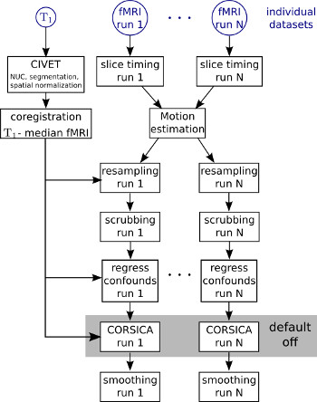
Before any statistical or pattern recognition model is applied on fMRI data, a number of preprocessing steps need to be applied. These steps first aim at reducing various artefacts that compromise the interpretation of fMRI fluctuations, e.g. physiological and motion artefacts. The second major aim is to align the data acquired at different points in time for a single subject, sometimes separated by years, and also to establish some correspondance between the brains of different subjects, such that an inference on the role of a given brain area can be carried at the level of a group. This page describes the steps of the NIAK preprocessing pipeline for fMRI (and T1) data. The pipeline includes most of the preprocessing tools currently available for connectivity analysis in fMRI: (1) Slice timing correction; (2) Estimation of rigid-body motion in fMRI runs, both within- and between sessions; (3) Linear or non-linear coregistration of the structural scan in stereotaxic space; (4) Individual coregistration between structural and functional scans; (5) Resampling of functional scans in stereotaxic space; (6) Scrubbing; (7) regression of confounds (average of white matter and CSF, motion parameters, COMPCOR); (8) Spatial smooting.

Syntax

The pipeline is invoked by niak_pipeline_fmri_preprocess. The argument files_in is a structure describing how the dataset is organized, and opt is a structure describing the options of the pipeline.

 niak_pipeline_fmri_preprocess(files_in,opt)

The structure files_in has an arbitrary number of fields, each one coding for a subject. Each subject field itself has two subfields fmri (describing all fMRI data available for this subject) and anat (describing one T1 data available for this subject). The fmri data field can have an arbitrary number of session subfields. A session correspond to a single acquisition of a single subject where only small movements are expected between brain volumes. Multiple runs are typically acquired within one session.

%% Subject 1
% T1 scan
files_in.subject1.anat = ...
   '/home/pbellec/demo_niak/anat_subject1.mnc';
% fMRI (motor)
files_in.subject1.fmri.session1.motor = ...
   '/home/pbellec/demo_niak/func_motor_subject1.mnc';
% fMRI (rest)
files_in.subject1.fmri.session1.rest = ...
   '/home/pbellec/demo_niak/func_rest_subject1.mnc';  

Labels for subjects, sessions and runs are arbitrary. To use special characters, for example a -, write files_in.('subject-1') instead of files_in.subject-1.

General options

The option opt.folder_out is used to specify the folder where the results of the pipeline will be saved. The pipeline manager will create but also delete many files and subfolders in that location.

opt.folder_out = '/database/data_demo/fmri_preprocess/';

The option opt.size_output can be used to adjust the quantity of intermediate results that are generated by the pipeline.

opt.size_output = 'quality_control';

Possible values are:

• 'quality_control': some outputs are generated at each step of the analysis for purposes of quality control. Intermediate steps are deleted as soon as they are no longer necessary.

• 'all': all possible outputs are generated at each stage of the pipeline.

Slice timing correction

In echo-planar imaging (EPI), the most common form of functional MRI sequences, different slices are acquired at different times. This can confound task-based regression analysis (especially with event-related designs), as well as connectivity analysis that rely on the correlation of fMRI time series located in different parts of the brain.

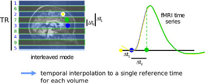
The slice timing correction is performed with niak_brick_slice_timing, and its options can be set in the pipeline using opt.slice_timing. The full list of option is available through the Matlab/Octave’s help command. This processing step is performing a temporal interpolation for each slice of each volume to a time of reference corresponding to one slice of reference of the volume. Specifying the parameters for slice timing correction essentially involves to specify the slice timing scheme (sequential or interleaved, ascending or descending), the scanner type (Siemens has sometimes a different way of defining interleaved) and the delay in TR. Note that the slice-timing correction is changing the timing of the acquisition. For this reason, a companion _extra.mat file is created for each fMRI dataset. This .mat file contains (amongst other things) a variable time_frames, with the time associated with each time frame (in the same unit as the TR, typically seconds).

 % Slice timing order. Available options:
 % 'sequential ascending'  , 'sequential descending',
 % 'interleaved ascending' , 'interleaved descending'
 opt.slice_timing.type_acquisition = 'interleaved ascending'; 

 % Scanner manufacturer.
 % Only the value 'Siemens' will actually have an impact
 opt.slice_timing.type_scanner     = 'Bruker';               

 % The delay in TR ("blank" time between two volumes)
 opt.slice_timing.delay_in_tr      = 0;

 % Skip the slice timing (0: don't skip, 1 : skip)
 opt.slice_timing.flag_skip        = 0;

Note that all of these infos are usually (but not always…) stored in the MINC header.

Type mincheader my_volume.mnc | grep acquisition in a shell terminal, and look at the section called acquisition.

The slice timing correction module is used to apply several minor additional operations. These additional operations need to be controlled through dedicated flags, independently from opt.slice_timing.flag_skip.

It is first possible to suppress “dummy” volumes. Dummy scans are the first volumes of an fMRI run, when the signal values have not yet stabilized. Modern scanners typically discard the dummy scans automatically. In doubt, it is better to suppress about 10 seconds of signal. For example, for fMRI data with a TR (inter-scan time) of 3 sec, the following option will remove 3 volumes (equivalent to 9s of scanning):

% Number of dummy scans to suppress.
opt.slice_timing.suppress_vol = 3;

Modern coils feature large number of channels (32 and more), which is associated with massive intensity inhomogeneities throughout the image. It is possible to apply an a posteriori (multiplicative) correction for these inhomogeneities, which may improve the T1-fMRI coregistration. This step is experimental, and should only be applied with caution.

% Apply a correction for non-uniformities on the EPI volumes (1: on, 0: of)
opt.slice_timing.flag_nu_correct = 1;
% The distance between control points for non-uniformity correction
% (in mm, lower values can capture faster varying slow spatial drifts).
% That parameter should be tweaked on an individual basis if large non-uniformities remain
% on the average functional volume
opt.slice_timing.arg_nu_correct = '-distance 200';

When the conversion from DICOM to NIFTI or MINC somehow did not work properly, the origin of the field of view can be very far from the center of the brain. This typically causes problems in coregistration steps. It is possible to ask NIAK to place the center of the field of view at the center of mass of the brain.

% Set the origin of the volume at the center of mass of a brain mask.
opt.slice_timing.flag_center      = 0;

Motion estimation

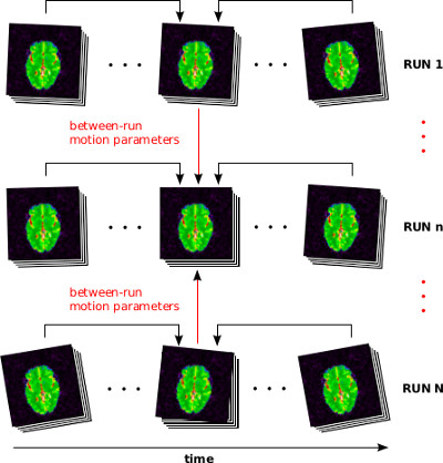
The motion of subjects over long period of time can cause severe misrealignement between fMRI brain volumes. Even small motion (say, less than one millimeter in translation or 1 degree in rotation) can cause substantial motion artefacts. A range of techniques exist to mitigate the impact of motion on fMRI time series, and it all starts by estimating the subject’s motion over time. This is done by estimating a rigid-body (three translation parameters, three rotation parameters) transform between each individual volume and one volume of reference (typically the median volume of the run). When multiple runs are acquired, possibly spread over multiple sessions, a single transformation is estimated across runs within session to a single reference run, and then a single transformation is estimated between sessions, using one session of reference.

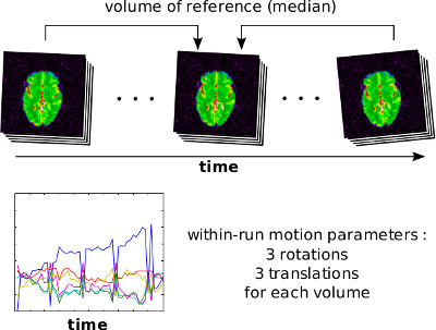
The motion of the subject during the fMRI runs is estimated using niak_pipeline_motion and its options can be set using opt.motion. The method is based on minctracc and performs a rigid-body registration of each fMRI volume to one volume of reference. The registration is actually performed on smoothed gradient images. The motion correction follows a hierachical strategy: (1) Rigid-body transforms are first estimated within each run independently by registering all volumes of the run to the median of the volumes. (2) The median volume of each run is coregistered to the median volume of a run of reference within each session. (3) The median volume of the runs of reference for all sessions are coregistered to the median volume of the run of reference of the session of reference. (4) The within-run, within-session and between-session estimates are combined to produce the final motion parameters.

A complete list of options for this brick can be found in the help of niak_pipeline_motion. The following example illustrates the most useful (or simply necessary) options.

% The session that is used as a reference.
% In general, use the session including the acqusition of the T1 scan.
 opt.motion.session_ref  = 'session1';

T1 normalization

To be able to automatically compare features of a given brain areas in the brain of many subjects, each individual brain is coregistered into a common stereotaxic space. By default, NIAK uses the MNI template, which is the average of 152 young healthy subjects. The coregistration is done first by linear transformation, i.e. translation, rotation and scaling, then a non-linear deformation is applied to correct for local differences in the volume and shape of brain areas.

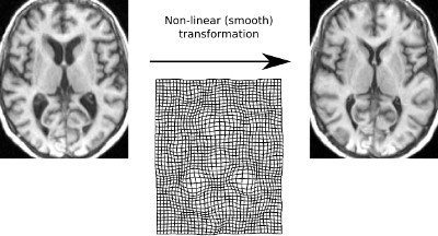
This step of the analysis is performed by niak_brick_t1_preprocess, and its options can be set using opt.t1_preprocess. This brick essentially implements the method for non-linear coregistration of a T1 scan in stereotaxic space found in the CIVET pipeline.

• Non-uniformity correction of the T1 image;

• Extraction of a brain mask; segmentation of the T1 image in white matter/grey matter/cerebrospinal fluid;

• Estimation of a linear and a non-linear transformation from the native T1 space to the MNI152 linear and non-linear stereotaxic space.

More details about the flowchart as well as a complete list of options for this brick can be found in the help of niak_pipeline_t1_preprocess. The following example illustrates the most useful (or simply necessary) option.

 % Parameter for non-uniformity correction.
 % 200 is a suggested value for 1.5T images, 75 for 3T images.
 % If you find that this stage did not work well, this parameter is usually critical to improve the results.
 opt.t1_preprocess.nu_correct.arg = '-distance 75'; 

BOLD-T1 coregistration

Even when acquired in the same session, the functional and structural scans need to be coregistered. Subjects indeed often move quite a lot between runs. This is a within-subject (rigid-body transform), between-modality (the images have inverted contrasts, amongst other differences) problem.

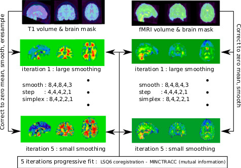
This step is implemented by niak_brick_anat2func, and its options can be set using opt.anat2func. The brick is based on minctracc and performs a rigid-body registration of a BOLD volume with a T1-weighted volume from a single subject. In the pipeline, the BOLD volume is the median of all fMRI volumes of the run of reference of the session of reference of each subject (as defined during the motion estimation). A complete list of options for this brick can be found in the help of ‘’niak_brick_anat2func’’.

Both volumes are corrected to have a zero mean inside their brain masks, and values outside the masks are set to zero. Those transformed volumes are then coregistered using an lsq6 transformation and a mutual information cost function following a “progressive fit” approach: the transformation is refined in 5 iterations using smaller bluring kernel and steps at each stage.

Spatial resampling

For each brain volume, the estimated parameters for motion with the run/session of reference as target are combined with the transformation from the run/session of reference (functional volume) to the structural volume, and then combined with the non-linear transformation to stereotaxic space. The functional brain volumes are resamples in one pass to the stereotaxic space using the combined (non-linear) transformation.

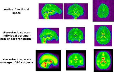
This step is performed by niak_brick_resample_vol, and its options can be set using opt.resample_vol. The brick is a simple overlay of the minc tool called mincresample. It is performing spatial resampling of 3D or 3D+t volumes, using a number of interpolation methods. A complete list of options for this brick can be found in the help of niak_brick_resample_vol. The following example illustrates the most useful (or simply necessary) option.

 % The resampling scheme.
 % The fastest and most robust method is trilinear.
 % Available options are: 'nearest_neighbour',
 % 'trilinear', 'tricubic', 'sinc'
 opt.resample_vol.interpolation = 'trilinear';

 % The voxel size to use in the stereotaxic space.
 opt.resample_vol.voxel_size = [3 3 3];

Regression of confounds

In order to reduce the influence of spatially structured noise on the fMRI time series, a number of confounds are regressed out from the time series using niak_brick_regress_confounds, after censoring of time points with an excessive amount of motion. The full list of options is accessible through Matlab/Octave’s help. Flags are avaible to turn on/off each group of confounding factors: slow time drifts, high frequencies, motion parameters, average signal of the white matter and ventricles, and the global signal. All the confounds are saved in the companion _extra.mat file that comes with every fMRI dataset, see the confounds and labels_confounds variables.

% 1: include the specified confounds in the regression,
% 0: exclude
opt.regress_confounds.flag_wm = 1;            
opt.regress_confounds.flag_vent = 1;
opt.regress_confounds.flag_motion_params = true;
opt.regress_confounds.flag_gsc = false;

Scrubbing Before any regression of confounds is implemented, the time frames with excessive motion are removed from the dataset following Power et al. (Neuroimage 2012). The censoring is based solely on one of the indices defined by Power and coll. (frame displacement, FD). Note that the scrubbing is changing the temporal grid of the dataset (i.e. some volumes are now missing). Most neuroimaging software will not handle these changes properly. In particular, if NIAK is used to preprocess dataset before a GLM analysis in another software package such as FSL or fMRIstat, it is important to skip scrubbing. A binary vector (named mask_suppressed) describing all the volumes that were removed from the original time series can be found in the _extra.mat companion file of each fMRI dataset. This includes the suppression of dummy scans from the slice timing correction as well as the scrubbing. The vector time_frames describe the time of each frame present in the dataset (i.e. excluding the volumes that have been removed).

% (1: apply scrubing / 0: don't apply)
opt.regress_confounds.flag_scrubbing = true;

% The threshold on frame displacement
% 0.5 is recommended
opt.regress_confounds.thre_fd = 0.5;

Slow time drifts/high frequencies A model of low-frequency temporal drifts as well as high frequency noise is generated using niak_brick_time_filter. The correction of slow time drifts is highly recommended because the frequencies below 0.01 Hz explain a large portion of the variance of the data, and mainly reflect motion artifacts. The correction of high-frequency noise is reducing the degrees of freedom of the time series without significant gain in SNR, so it is in general not advisable. It still seems to be common practice to filter out frequency above 0.08 Hz is the resting-state community, but this is not the default parameter in NIAK.

 % Cut-off frequency for removal of low frequencies (in Hz).
 % A cut-off of -Inf will result in no high-pass filtering.
 opt.time_filter.hp = 0.01;

% Cut-off frequency for removal of high frequencies (in Hz).
% A cut-off of Inf will result in no low-pass filtering.
opt.time_filter.lp = Inf;

Motion parameters The 6 rigid-body motion parameters (3 translations and 3 rotations) are not entered as such in the model. First a twelve parameters model is built by including the original 6 parameters as well as their square (Lund et al. 2006, reference below). Then a principal component analysis is used to retain 95% of the variance of these twelve parameters, which typically entail around 8 covariates but may vary from dataset to dataset.

White matter & ventricular signals The masks of the ventricle and the white matter have been built to be very conservative. This is to avoid getting influenced by the surrounding grey matter tissue maps (see Saad et al. 2012, reference below), in which case the average of the white matter mask becomes highly correlated with the global average.

Global signal The global average estimator is not the traditional estimator, but rather the estimator based on a principal component analysis as described in (Carbonell et al. 2012, reference below). This estimator alleviates some of the theoretical limitations of the classical estimator, as reported by Murphy et al., 2010 (reference below). However, as this correction may introduce some bias in the group comparison (Saad et al. 2012), the regression of the global average is turned off by default.

Spatial smoothing

The application of spatial smoothing has the potental to slightly increase the signal-to-noise ratio, and also mitigate the impact of misregistration between functional areas, that were not perfectly aligned across subjects by the non-linear coregistration in stereotaxic space.

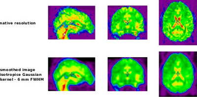
The spatial smoothing is performed using niak_brick_smooth_vol, and its options can be set using opt.smooth_vol. The brick is a simple wrapper of the minc tool called mincblur. It is implementing spatial smoothing using a Gaussian kernel. A complete list of options for this brick can be found using Matlab/Octave’s help. The following example illustrates the most useful (or simply necessary) options.

% Field width at half maximum of the bluring kernel
opt.smooth_vol.fwhm = 6;
% Skip spatial smoothing (0: don't skip, 1 skip)
opt.smooth_vol.flag_skip = 0;

Tuning individual parameters

It is not generally possible to process successfully all subjects in a dataset with the same parameters. Please refer to the quality control manual for a list of what outputs to check and how to fix problems. The following mechanism can be used to change the parameters of individual subjects:

opt.tune(1).subject = 'subject1';
opt.tune(1).param.slice_timing.flag_center = true;

opt.tune(2).subject = 'subject2';
opt.tune(2).param.slice_timing.flag_center = false;

Here the parameters of the slice timing will be tuned specifically for subject1 and subject2. Anything that usually goes in opt can go in param. The parameters specified in opt apply by default, but will be overridden by tune.param. Specifically, in that example, all the parameters specified for opt.slice_timing will still apply for subject1 and subjec2, except for flag_center that will be set to true for subject1, and false for subject2.

Publication guidelines

Here is a short description of the fMRI preprocessing pipeline that can be adapted in a publication. You are encouraged to include the script that was used to preprocess the fMRI database as supplementary material of the article.

The fMRI database was preprocessed using the Neuroimaging Analysis Kit (NIAK) release 0.12.4 (Bellec et al. 2011, NIAK website). The three first volumes of each run were suppressed to allow the magnetisation to reach equilibrium. Each fMRI dataset was corrected of inter-slice difference in acquisition time and the parameters of a rigid-body motion was estimated for each time frame. Rigid-body motion was estimated within as well as between runs. The median volume of one selected fMRI run for each subject was coregistered with a T1 individual scan using Minctracc (Collins et al. 1997), which was itself non-linearly transformed to the Montreal Neurological Institute (MNI) template (Fonov et al 2011) using the CIVET pipeline (Ad-Dab’bagh et al. 2006). The MNI symmetric template was generated from the ICBM152 sample of 152 young adults, after 40 iterations of non-linear coregistration. The rigid-body transform, fMRI-to-T1 transform and T1-to-stereotaxic transform were all combined, and the functional volumes were resampled in the MNI space at a 3 mm isotropic resolution. The “scrubbing” method of Power et al., 2012, was used to remove the volumes with excessive motion (frame displacement greater than 0.5). The following nuisance parameters were regressed out from the time series at each voxel: slow time drifts (basis of discrete cosines with a 0.01 Hz high-pass cut-off), average signals in conservative masks of the white matter and the lateral ventricles as well as the first principal components (95% energy) of the six rigid-body motion parameters and their squares (Lund et al. 2006, Giove et al. 2009). The fMRI volumes were finally spatially smoothed with a 6 mm isotropic Gaussian blurring kernel. A more detailed description of the pipeline can be found on the NIAK website.

Relevant references for the fMRI preprocessing pipeline are listed below.

Regarding the NIAK package

P. Bellec, F. M. Carbonell, V. Perlbarg, C. Lepage, O. Lyttelton, V. Fonov, A. Janke, J. Tohka, A. Evans, A neuroimaging analysis kit for Matlab and Octave. Proceedings of the 17th International Conference on Functional Mapping of the Human Brain, 2011.

The documentation of the NIAK package.

Online NIAK fMRI preprocessing documentation. http://niak.simexp-lab.org/pipe_preprocessing.html

On the minctracc coregistration tool.

Collins, D.L. Evans, A.C. (1997). “ANIMAL: Validation and Applications of Non-Linear Registration-Based Segmentation”. “International Journal of Pattern Recognition and Artificial Intelligence”, vol. 11, pp. 1271-1294.

On the “scrubbing” method.

J. D. Power, K. A. Barnes, Abraham Z. Snyder, B. L. Schlaggar, S. E. Petersen. Spurious but systematic correlations in functional connectivity MRI networks arise from subject motion. NeuroImage Volume 59, Issue 3, 1 February 2012, Pages 2142–2154

On the MNI ICBM152 young adult symmetric non-linear 50 iterations template

VS Fonov, AC Evans, K Botteron, CR Almli, RC McKinstry, DL Collins and the brain development cooperative group. Unbiased average age-appropriate atlases for pediatric studies. NeuroImage, Volume 54, 2011, pp. 313-327. http://www.bic.mni.mcgill.ca/ServicesAtlases/ICBM152NLin2009

On the CIVET pipeline.

Ad-Dab’bagh, Y., Einarson, D., Lyttelton, O., Muehlboeck, J.-S., Mok, K., Ivanov, O., Vincent, R.D., Lepage, C., Lerch, J., Fombonne, E., and Evans, A.C. (2006). The CIVET Image-Processing Environment: A Fully Automated Comprehensive Pipeline for Anatomical Neuroimaging Research. In Proceedings of the 12th Annual Meeting of the Organization for Human Brain Mapping, M. Corbetta, ed. (Florence, Italy, NeuroImage). Poster.

Regarding the method for non-uniformity correction of the structural scan.

Sled, J.G., Zijdenbos, A.P., and Evans, A.C. (1998). “A Nonparametric Method for Automatic Correction of Intensity Nonuniformity in MRI Data”. IEEE Transactions on Medical Imaging 17, pp. 87-97.

Regarding the brain extraction on the structural scan.

J. G. Park, C. Lee (2009). “Skull stripping based on region growing for magnetic resonance brain images”. NeuroImage 47(4):1394-1407.

Note that the actual algorithm used in NIAK was only inspired by this last paper.

A more detailed description can be found in the help of niak_brick_mask_brain_t1.

Regarding partial volume effects.

Tohka, J., Zijdenbos, A., and Evans, A.C. (2004). “Fast and robust parameter estimation for statistical partial volume models in brain MRI”. NeuroImage, 23(1), pp. 84-97.

Regarding the estimation of the global signal.

F. Carbonell, P. Bellec, A. Shmuel. Validation of a superposition model of global and system-specific resting state activity reveals anti-correlated networks. Brain Connectivity 2011 1(6): 496-510. http://dx.doi:10.1089/brain.2011.0065

Regarding regression of confounds in fMRI.

Lund, T. E., Madsen, K. H., Sidaros, K., Luo, W.-L., Nichols, T. E., Jan. 2006. Non-white noise in fMRI: does modelling have an impact? NeuroImage 29 (1), 54-66. http://dx.doi.org/10.1016/j.neuroimage.2005.07.005

F. Giove, T. Gili, V. Iacovella, E. Macaluso, and B. Maraviglia. Images-based suppression of unwanted global signals in resting-state functional connectivity studies. Magnetic Resonance Imaging, 27(8):1058–1064, 2009.

Regarding the impact of global signal regression for group comparison.

Saad, Z. S., Gotts, S. J., Murphy, K., Chen, G., Jo, H. J. J., Martin, A., Cox, R. W., 2012. Trouble at rest: how correlation patterns and group differences become distorted after global signal regression. Brain connectivity 2 (1), 25-32. URL http://dx.doi.org/10.1089/brain.2012.0080

Regarding the pipeline system for Octave and Matlab (PSOM).

P. Bellec, S. Lavoie-Courchesne, P. Dickinson, J. Lerch, A. Zijdenbos, A. C. Evans. The pipeline system for Octave and Matlab (PSOM): a lightweight scripting framework and execution engine for scientific workflows. Front. Neuroinform. (2012) 6:7. Full text open-access: http://dx.doi.org/10.3389/fninf.2012.00007